Blade Runner

Usually the task of a performance engineer involves running a workload, finding its first bottleneck with a profiling tool, eliminating it (or at least minimizing it), and then repeating this cycle – up until a desired performance level is attained. However, sometimes the question is posed from the reverse angle: Given existing code that requires a certain amount of time to execute (e.g., 10 minutes), what would it take to run it 10 times faster? Can it be done? Answering these questions is easier than you would think.

Parallel Processing

The typical parallel computing workload breaks down a problem in discrete chunks to be run simultaneously on different CPU cores. A classic example is approximating the value of pi. Many algorithms that numerically approximate pi are known, variously attributed to Euler, Ramanujan, Newton, and others. Their meaning, not their mathematical derivation, is of concern here. A simple approximation is given by Equation 1.

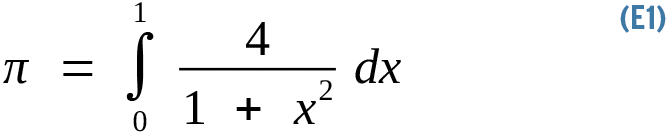
The assertion is that pi is equal to the area under the curve in Figure 1. Numerical integration solves this equation computationally, rather than analytically, by slicing this space into an infinite number of infinitesimal rectangles and summing their areas. This scenario is an ideal parallel numerical challenge, as computing one rectangle's area has no data dependency whatsoever with that of any another. The more the slices, the higher the precision. You just need to throw CPUs at the problem: in this case, 5 million loops to reach 48 decimal places of accuracy.

This way of approximating pi is not very efficient, but it uses a very simple algorithm to implement in both linear and parallel coding styles. Carlos Morrison published a message passing interface (MPI) [1] pi implementation [2] in his book Build Supercomputers with Raspberry Pi 3 [3].

Speed Limit

Can you make the code twice as fast? Sure! Can you make it 10 times faster? Maybe. That factor, 2x or 10x, is called speedup in computing (Equation 2).

Speedup is defined as the ratio of the original and new (hopefully improved) measurements, so if your code used to take one second to execute and now takes half a second, you have a 2x speedup. Speedup measures for latency or throughput – today I am using the latency formulation.

Amdahl's law [4] observes that parallelism only accelerates a fraction of the application's code, putting a limit on its effect. Ideally, speedup would be linear, with a doubling of processing resources consistently halving the compute time, and so on indefinitely. Unfortunately, few algorithms can deliver on this promise (see the "Embarrassingly Parallel Algorithms" box); most algorithms approximate linear speedup over a few CPUs and essentially decay into constant time with many CPUs.

For example, if your code takes 20 minutes to execute and just one minute of it can't be parallelized, you can tell up front, without knowing any other details about the problem, that the maximum speedup theoretically possible is 20x (Equation 3),

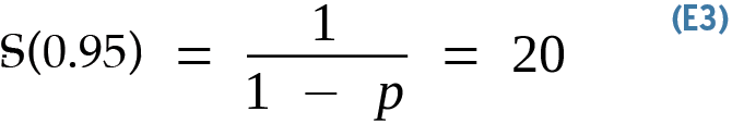
which is derived by observing that you can use as many CPUs as you want to drive 95 percent of the problem asymptotically to zero time (p=0.95), and you will be left with that one minute (1 – p=0.05). Once you do the math (1/0.05=20), that is the maximum possible speedup under ideal conditions (i.e., the absolute limit with infinite resources thrown at the problem).

Amdahl's Law

IBM's Gene Amdahl contributed the law bearing his name in 1967, coupling the previous observation with the simple fact that you generally do not have infinite horsepower to drive the parallel section of the code to zero time (Equation 4).

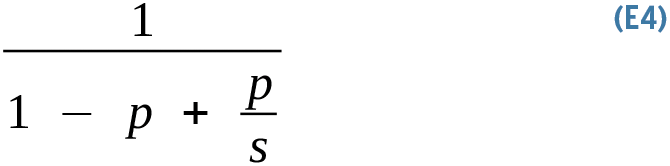
Amdahl's observation factors in the speedup of the parallel section. The new term p/s is the ratio of time spent in the parallel section of the code and the speedup it achieves.

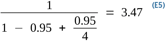
Continuing with the 20-minute example, say you have accelerated the now-parallel section of the code with a 4x speedup, and you find that the resulting speedup for the whole program is 3.47x (Equation 5):

There are some important observations to be made here. First, accelerating code is usually about removing bottlenecks, not absolute speedup numbers for the whole codebase. Second, given more resources, you will usually process more data or do more work. Gustafson's law [6] provides an alternative formulation: If more resources are made available, larger problems can be solved within the same time, as opposed to Amdahl's law, which analyzes how a fixed workload can be accelerated by adding more resources. Keep these points in mind and remember that, in the real world, network communication is always a distributed system's presumptive bottleneck.

Roy Batty's Tears

The power of Amdahl's law is found in its analytical insight. Code is measured in time, not in lines, so some minimal performance testing is still required. If you determine that only 50 percent of an algorithm's critical section can be parallelized, its theoretical speedup can't exceed 2x, as you see in Figure 2. Furthermore, it's not practical to use more than 12 cores to run this code, because it can attain more than 90 percent of the maximum theoretical speedup with 12 cores (a 1.84x speedup). You know this before attempting any optimization, saving you effort if the best possible result is inadequate to achieving your aims.

In an alternative scenario with only five percent serial code in the bottleneck (Figure 3), the asymptote is at 20x speedup. In other words, if you can successfully parallelize 95 percent of the problem, under ideal circumstances the maximum speedup for that problem is 20x. This handy analysis tool can quickly determine what can be accomplished by accelerating code for a problem of fixed size.

Without invoking the C-beams speech or even going near the Tannhäuser Gate [7], one must point out parallelism's massive overhead, already obvious from the examples here. Execution time can be significantly reduced, yet you accomplish this by throwing resources at the problem – perhaps suboptimally. On the other hand, one could argue that idle CPU cores would not be doing anything productive. All those cycles would be lost … like tears in rain.