Tech-Speak

The Python programming language is wildly popular because it's easy to write, easy to read, and can be made to do almost anything with its huge stack of libraries. Yet, one complaint is heard over and over: It's too slow! This drawback might not matter much for web programming, where your program can spend more time waiting for responses from the network and database than actually computing anything, but data scientists, physicists, and engineers who try to use Python for real number crunching quickly hit the performance wall. A new language called Julia promises to be as easy to program as Python and other dynamic, interpreted languages, while offering the execution speed of statically typed, compiled languages such as C and Fortran.

Dynamic Languages

The popularity of interpreted, dynamically typed languages is easy to understand. You can get right to the real work in your program without spending multiple lines of code on ceremony and bookkeeping. You don't need to declare data types, manage memory, or think about how your high-level code will be translated into machine instructions. Perhaps best of all, you can type expressions into an interactive prompt, often called a REPL (read-eval-print loop), and get immediate results. The REPL allows you to experiment freely, try out ideas, and use your favorite programming language as a sophisticated calculator.

These types of dynamic languages used to be called "scripting languages," because they were used in shell scripting; however, as their applications have grown far beyond their original niche in automating system maintenance tasks, this term is falling out of use. These days Python, Ruby, R, Perl, and other languages in this class are grouped together under various and sometimes inaccurate terms. In this article, I adopt the description "dynamic languages" to reflect the dynamic nature of their data typing. (See also the "Common Confusion" box.)

Static Languages

The other major class of languages are statically typed: C, Fortran, Java, C++, and others. In these programming languages, the type of every variable is fixed before compilation, either explicitly or by convention or inference, and a particular variable cannot be used for more than one major type. These languages have no REPL: Your program needs to be compiled as a whole and linked with any external resources it references each time you change it. Therefore, they cannot be used interactively. Exploration or program development thus involves many cycles of edit-compile-run.

Some people extol static typing as a way to avoid many classes of programming errors or to expose them during compilation before running the program. Others consider it annoying ceremony, getting in the way of the real business of expressing an algorithm in code. It's partly a matter of taste and partly experience. One objective advantage of static typing is that it allows the compiler to produce more optimized, and therefore faster code, which is one of the reasons languages such as Fortran and C are still the workhorses [1] of large-scale computing and simulation in demanding disciplines such as weather forecasting, physics research, and economic modeling.

Dynamic Problems

Nevertheless, the convenience of dynamic, interactive languages is tempting enough that scientists and engineers have tried to bend them to their purposes. Python, for example, has become popular with data scientists in recent years. How do these computational scientists overcome the intrinsically poor performance of these languages? Several techniques can speed up dynamic languages, but most of them come down to rewriting the time-consuming parts of the code in one of the fast static languages or using pre-built libraries (e.g., NumPy [2] for Python) that call on Fortran or C routines to do common tasks in array manipulation, linear algebra, and the like.

This setup leads to two-language problems [3]: Your program is now written in a mix of languages with incompatible paradigms; you need to manage the interface between languages; you may wind up on large projects with different teams specializing in the different languages; and the overhead of calling foreign functions may eat in to the gains in execution speed, depending on the efficiency of your language's foreign function interface. Moreover, your code becomes more difficult to read, develop, and maintain.

If you are fortunate enough that big parts of your problem can be passed off to NumPy or a similar library, parts of your calculation will still need to be expressed in the host language and will remain slow. Also, a library written in a foreign language will typically bind you to a particular implementation of your dynamic language, limiting your choices in the future.

Julia

The Julia [4] language was intended to offer an alternative to the two-language problem. It has an elaborate type system but can be used as a simple, dynamically typed language with an intuitive, expressive syntax. It has a REPL with helpful features, such as built-in help and package management systems. It can interface directly with graphics libraries, as you'll see, to produce scientific visualizations directly from your code; yet, it achieves execution speeds on par with Fortran and C [5].

Since its first beta release in 2012, these qualities have attracted a growing community of numerical scientists to the young language. Naturally, Julia love is not unanimous, but the general agreement is that it has met its ambitious goals and represents the fulfillment of a long-held desire for a language that is as fast as Fortran but as easy as Python.

Given that, Julia's first stable release version 1.0 in August 2018 was a milestone for the technical computing community. The main significance of this release is a promise of language and API stability for the long term, allowing users to undertake major projects, knowing that changes to the language will not require any changes to code under development. The original language design arose from academic computer science research at MIT conducted by Alan Edelman, Stefan Karpinski, Jeff Bezanson, and Viral Shah.

Julia Syntax

This article will not be a complete tutorial for the Julia language, but I will demonstrate the main language features and give you a feel for its syntax, which should allow you to get started experimenting with the language and give you a good idea of whether you might want to consider adopting it for your next project.

First, you need to install Julia. To get the latest version, go to Julia headquarters [4] and click on the prominent Download button. At the time of writing, that got me version 1.0.1, on which the code examples in this article, executed on a Linux laptop, are based. A source download and binaries are available for Linux, macOS, Windows, and BSD.

Installation from the binary packages is simple, because all of the dependencies to get started are included. After installing, type julia at the terminal; you will see a welcome message, and your shell prompt should change to julia>. Now you can type Julia expressions and see the results. Try typing 1 + 1; or, type 1 + "s" to see what a type error looks like.

Those examples used numbers and strings. Before getting deeper into syntax, I'll take a brief look at Julia's other data types. Strings, enclosed in double quotation marks, are made up of sequences of characters. Individual characters are enclosed in single quotes (e.g., 's'). Therefore, "st" is a valid string, but 'st' is a syntax error. The operator for string catenation is *, which is one of Julia's syntax oddities, but one for which they have a detailed, theoretical argument (which need not concern us here). You can stick strings and characters together to get longer strings; for example, "str" * 'i' * "ng" yields "string".

Julia has several types of numbers. In addition to integers, you can compute with floating point numbers, integers with arbitrary precision, complex numbers, and rational numbers (notated <numerator>//<denominator>). You must know how your language of choice handles integers, as shown in Table 1, to avoid the "integer division pitfall."

Listing 1 contains part of a Julia interactive session that shows how Julia's rational numbers work. One interesting feature of this number type is that Julia represents each rational number internally in its reduced form, which explains the results of the call to the numerator() function.

julia> 1//2 + 1//3
5//6
julia> numerator(10//12)
5
julia> 2//3 == 4//6
true
julia> 2//3 == 4/6
false

After strings and the various types of numbers, the most important built-in data type in Julia is the array. Any significant computation in the language will involve extensive use and manipulation of arrays, and Julia is designed to make this easy and expressive. Arrays are defined by square brackets, and you can glue them together horizontally with a space or vertically with a semicolon, as shown in Listing 2 (ending a line with a semicolon suppresses the printing of the result in the REPL).

julia> a = [1 2];
1x2 Array{Int64,2}:
 1  2
julia> b = [3 4];
1x2 Array{Int64,2}:
 3  4
julia> [a b]
1x4 Array{Int64,2}:
 1  2  3  4
julia> [a; b]
2x2 Array{Int64,2}:
 1  2
 3  4
julia> [a' b']
2x2 Array{Int64,2}:
 1  3
 2  4

In Listing 2, note that the prime operator (') transposes an array. Julia has many operators that act on arrays as a whole. Some of the most useful ones are reshape(A, dimens), which reforms the elements of A into a new shape specified by dimens; rand(dimens), which creates a new array and fills it with random numbers; and range(start, stop=stop, length=n), a convenient way to create an evenly spaced set of numbers, which is useful in graphing. Additionally, Julia's linear algebra library provides a host of mathematical operations on 2D arrays, providing ways to factor, calculate eigenvalues and eigenvectors, perform inverses, and do all the usual math on matrices.

The ability to operate on arrays as units or extend operations elementwise over an array is a part of the language syntax that allows you to express many complicated calculations without writing loops. Julia uses a dot (.) that extends a function or binary operator to operate element-by-element over an array. For example, a .+ b returns the array [4 6], which is 1+3 2+4, and a .* b gets you [3 8] (1*3 2*4). However, if you omit the dot, you will get the matrix product of the two arrays; so a * b' returns a matrix with the single element 11.

Julia uses the dot syntax to extend any function, so it can operate efficiently over arrays – and this extends to functions that you define yourself. For example, sin.(a) returns the array [0.841471 0.909297], which is [sin(1) sin(2)]. If you chain together dotted functions, as in the expression cos.(sin.(a)), the Julia compiler "fuses" the operations: Rather than applying the sine function to the array, and then the cosine function to the resulting array, the combined function is applied once per array element. This strategy is one of many that the compiler applies to make array operations space and time efficient, and it works with any combination of operators and built-in or user-created functions.

Julia has several other major built-in data types familiar from other modern languages, including tuples and dictionaries, but it also goes further and offers a flexible and sophisticated type system that includes user-defined types. These can be as elaborate as you like and can inherit behaviors from built-in or other user-defined types, yet they are treated equivalently to built-in types by the compiler, which means their use does not hinder optimization.

Type declarations are optional in Julia. They can sometimes help the compiler optimize your code but are generally not required for this purpose. Julia is strictly typed, but the compiler will infer the types of your variables if you do not declare them. As you design your program, you will mainly use types to organize your code and data and to express your algorithm more naturally, rather than to help the compiler generate more efficient machine instructions. As a beginner with the language, you can certainly get by with a sparse use of declarations involving only the built-in types and learn how to employ the more advanced capabilities of the type system as you gain expertise.

Listing 3 shows Julia's basic control structures, most of which are fairly conventional. Indentation is for convention and readability and is not part of the syntax. The end statements that terminate each block are required, however.

# while loop
i = 1;
while i < 7
  print(i^2, "; ")
  global i = i + 2
end
# for loop using iterators
for n in 1:5
  print(2^n, "--")
end
# implied nested loop
for i = 1:2, j = 1:2
  println([i, j])
end
# loop over container
for i in ["first", "second", "third"]
  println(i)
end

The four examples are annotated with the # syntax for a single-line comment (multiline comments start with #= and end with =#). The results of most of these examples should be easy to predict, but the best way to learn this or any language is, of course, to try things out yourself.

One quirk is illustrated in the first example: Blocks in Julia create a local scope, so variables need to be distinguished with the global or local keywords.

The implied nested loop shown in Listing 3 is a convenient syntax shortcut that removes the need for repetitive and deeply nested loop structures when looping over multiple variables, something ubiquitous in numerical code.

Unicode

Almost all languages in wide use today were created before the advent of Unicode, the universal standard that finally allowed working with computers in any of the world's writing systems and included a host of special symbols. Because of this history, most existing languages have at best an awkward relationship with the world of Unicode. Those that have mature Unicode support have gained it though a painful process of radical language revision, as in the transition from Python 2 to Python 3.

Julia has the advantage of having been designed after Unicode was universally accepted, and it embraces this powerful and liberating technology fully by defining characters and strings in terms of Unicode by default. You are also free to include any Unicode characters in the names of variables, functions, and operators, and some of Julia's built-in operators have Unicode versions to match the symbols used in mathematical writing. For example, you can write the final example in Listing 3 as

with the mathematical symbol for membership in a set. If you have no convenient way to enter this symbol, you can take advantage of another of the REPL's special features: support for entering special symbols with LaTeX syntax. To get this symbol, type \in and press the Tab key (\in<TAB>), and the REPL inserts for you.

The ability to construct variable names out of Unicode allows you to incorporate subscripts and superscripts into variable names, so you're able to make fewer typographic compromises when translating mathematical formulas into computer code. Another detail of Julia's syntax interprets a number prepended to a variable to signify multiplication, just as in conventional mathematical notation, with no explicit multiplication sign required. Combining these typographic conveniences allows you to write legal Julia expressions such as

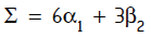
by using LaTeX notation \alpha<TAB>\_1<TAB> and \beta<TAB>\_2<TAB> for the Greek letters with subscripts.

The Package System

Julia has its own sophisticated package management system that allows you to import libraries of code from an official repository, manage personal or private group repositories, and bundle projects with their dependencies to avoid the dreaded "dependency hell" that so often besets the modern software developer. A "package" in Julia is a project of one or more files containing code with certain functions designed for export into other projects.

Here I'll concentrate on using the package system to import public libraries that add functionality. The package system is such an integral part of the Julia environment that the REPL has a special mode for working with packages, which you enter by typing a right square bracket (]). You can also use normal language commands, which is the style I cover here, because these are the commands that you can use in saved programs.

The package system is part of the standard library but must be imported before you can use it. To make it available in the REPL or in your programs, you must say using Pkg first. This is the case as well with many other parts of the included standard library that are not loaded by default, which helps the interpreter start up quickly and saves resources. For example, before you can use the linear algebra functions mentioned in the previous section, you must import them with using LinearAlgebra.

After importing the Pkg library, you can use it to download the packages you want to use in your projects but that are not yet installed on your system. Entering the command

Pkg.add("<packagename>")

will, by default, download the specified files from the official repository and install them on your system – or upgrade the package if it's already present.

The first time you import the new functions with the using command, you will experience a delay while they are precompiled, after which their names are available in the current namespace. If you prefer to keep the imported names in their own namespace, use the command import <modulename> instead, after which you must refer to the imported names as <modulename>.<function>.

You can browse more than 1,900 packages at a centralized registry [6], which contains an impressive variety of software, ranging from serious scientific and math packages to programs for automating Minecraft. However, the status of these packages varies widely: Although many of them are mature, others are experimental or in the early stages of development. Also, the recent release of the stable version of Julia contained some changes to syntax that broke many existing packages, and as of this writing, a good deal of software in the repository still will not compile.

Graphing

Most of the packages in the ecosystem serve specialized interests, but many users will eventually be interested in visualizing their results. Therefore, a closer look at some of Julia's graphing packages is likely to be of general interest. Although you have several from which to choose, the most widely used graphing package, and most flexible, is the package that you acquire with the command:

Pkg.add("Plots")

This plotting meta-system of sorts allows you to use several plotting back ends with a unified syntax and attempts, its author claims, to understand your intentions and produce the plot you want using the capabilities of the back end you specify. I'll show you how this works with some examples.

After fetching the package, you need to import it before you can use it. The command for this is simply using Plots. If you have not used Plots before, this command will initiate a precompilation, with messages on the terminal if you are using the REPL. Subsequent plot commands will be executed by the default plotting back end, which turned out in my recent tests to be GR, but the default seems to change over time and may be something else by the time you try this out.

GR is a very capable plotting system, providing fast generation of a wide variety of visualizations. To ask Plots which back end is currently selected, simply type backend() at the REPL prompt. Below are several examples showing how to use the Plots system, with the results as generated by the GR back end. The beauty of this package is that you can change the back end merely by invoking its name in lowercase, and these plot commands will all work unchanged, with the plots rendered by the back end you select.

Without changing your code, you can experiment with different back ends to find the one that produces the best output for your particular plot. You can also use, for example, the package UnicodePlots, which renders plots right to the terminal, for a quick look at your data, and switch to another back end when it's time to produce graphs for publication.

Most back ends don't come with the Plots package, which means you'll need to download and import them separately. For instance, to make terminal plotting available, download, import, and switch to the package with

Pkg.add("UnicodePlots")
using UnicodePlots
unicodeplots()

The basic command for creating a line plot from a function is:

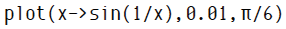
With the Plots system activated, as described above (if you entered using UnicodePlots above, revert to Plots with using Plots before proceeding), a window should pop up resembling Figure 1; if you're using a back end different from GR, it will appear somewhat different. A considerable delay takes place before the first plot in a session appears, but subsequent plots appear more quickly. This example also serves to illustrate Julia's convenient syntax for defining an anonymous function used in the first argument; the second and third arguments define the domain along the x axis.

If you execute additional plot commands, each new plot replaces the existing plot. If, instead, you want to add something to the current plot, use the version with an exclamation mark,

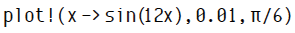
to add the new function to the existing plot (Figure 2).

In this way, you can incrementally build up the plot you want. When you decide to save your masterpiece in a file, use the command savefig("figure1.pdf"). This will save a PDF of the last plot you made, which is a good choice for high-resolution reproduction. Plots supports many file types, depending on the back end. GR can save plots as PNG, SVG, and PostScript, as well; specify your choice by the filename extension.

The Plots package with the GR back end supports many other types of graphs. The commands

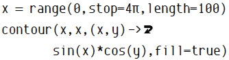
produce the filled contour plot shown in Figure 3. To begin, create a set of equally spaced coordinates; the first command shows Julia's convenient syntax for doing that. The second command plots the contours with the two-variable version of anonymous function definition.

Multiple Dispatch

Rather than encouraging the programmer to use classes and objects to organize code, Julia combines its type system with function definition to create an organizing principle that pervades the language and its standard library. To understand how this works, you first need to learn how to define functions.

Listing 4 defines a function called addcat. In fact, as you can see, it defines it twice. Each definition uses type annotations in its list of arguments. The first version accepts two numbers (of any kind) and returns their sum. The second version accepts two strings and returns them joined together and separated by a space. When you call this function, the compiler looks at the type of arguments supplied and uses the version that is most specific to those arguments. This mechanism is called "multiple dispatch," because the version that is dispatched, or called, depends on all of the arguments supplied, rather than, for example, only the first, which is the usual way functions are dispatched in object-oriented languages.

function addcat(a::Number, b::Number)
  return a + b
end
function addcat(a::String, b::String)
  return a * " " * b
end

In this way, you can define a set of possible behaviors for your functions as wide as you need, without writing assertions or type-checking code. This method becomes even more powerful if you combine the multiple dispatch mechanism with user-defined types.

To see the entire list of versions, or "methods," defined for a function, you can type methods(<function>). If you ask, for example, for methods(sin), you will see a list of 12 methods defined for this trigonometric function, written to handle floats, complex numbers, and various types of arrays. If you want, you can also admire the list of 376 versions of the multiplication operator (*).

The Future of Scientific Computing

Julia was designed with the scientific and technical numericist in mind. I've only had space to scratch the surface of what this young language offers to the programmer who requires the generation of highly efficient code but would also like to take advantage of the sophisticated abstractions offered by modern, high-level dynamic languages.

To this end, Julia incorporates a complete metaprogramming system, including powerful, Lisp-like macros, an elaborate type system, the ability to examine generated machine instructions, and more. Its facilities for parallel and distributed computing, which are part of its standard library, are unmatched in their ease of use, allowing you to take advantage of multiple cores on a single machine, supercomputing clusters, or a heterogeneous network of computers with almost no additional code. For more information on these topics, the extensive online manual [7] is a good place to start, although after the first few chapters, its explanations can become far too terse. Fortunately, the Julia community page [8] contains a good list of resources for help and information.

Julia is a free software success story developed in the open, on GitHub, with more than 700 contributors, many of whom are the scientists and engineers who use the language in their research. It is in use at hundreds of universities and companies and, especially after its 1.0 release, is experiencing rapid adoption [9] by a community of enthusiastic users.

Julia may represent the holy grail of a language that does not compromise in performance, while demanding no more of the programmer than a dynamic scripting language and offering the sophisticated user the fruits of academic computer science. Julia may represent what was once thought impossible: a language that is as easy as Python but as fast as Fortran.